Weather Station Hack
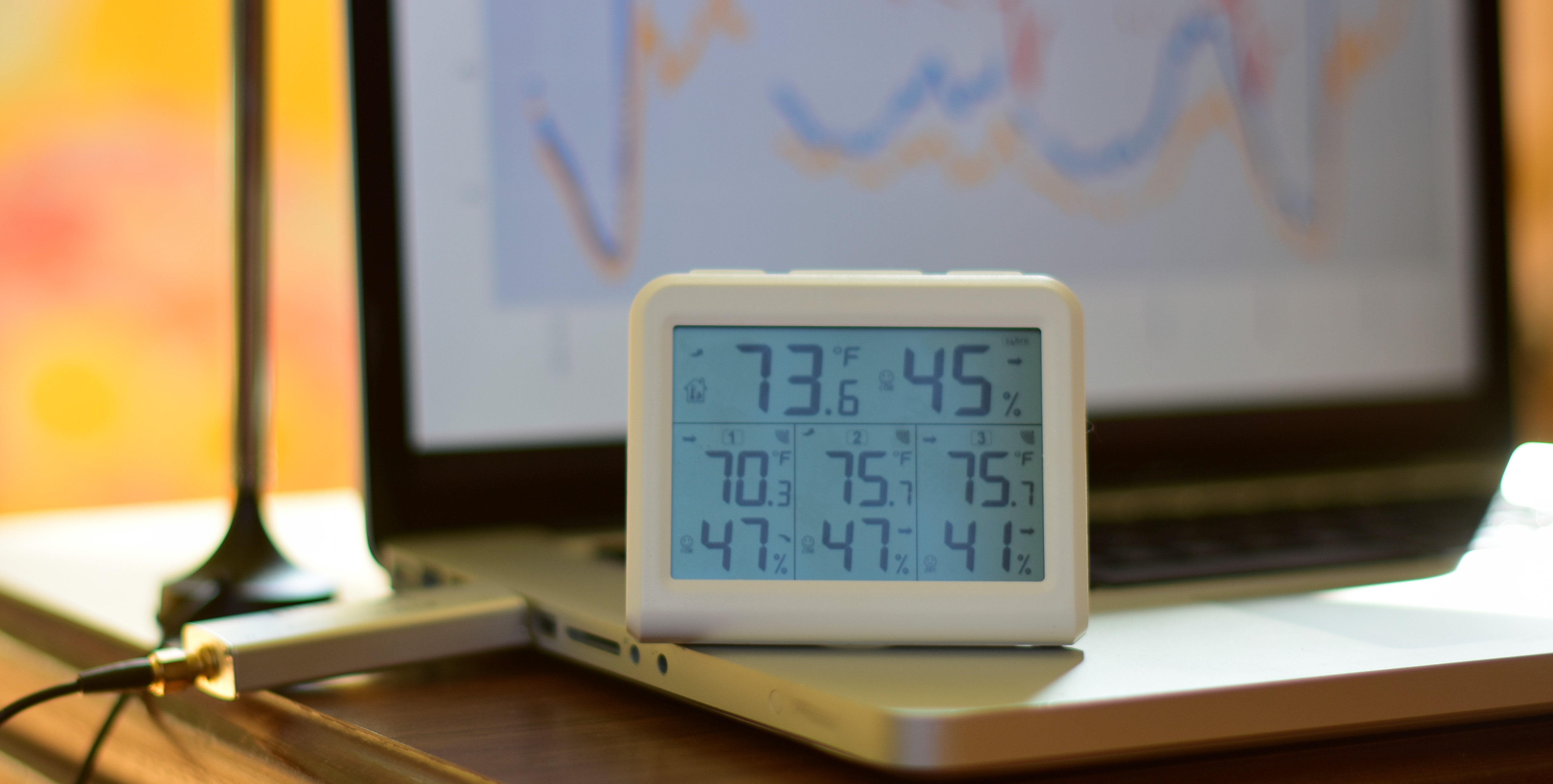
I’ve had this wireless digital thermometer/hygrometer for a while now and we keep it in our kitchen so we can quickly see the temperature outside and know how to dress the kids and if they need snow pants or just a light jacket or if it is warm enough to run around in the sprinklers as was the case today. The device came with 3 sensors which I have located in a few places throughout the house.
Software Defined Radio
I have also had a software defined radio RTL-SDR dongle laying around that I experimented with a few years ago. I had fun trying to listen in on ham radio communications and a few shortwave stations.
Earlier this week, I was wondering if I could see the signal coming from my cheap weather station. It turns out that 433Mhz is a standard frequency for these and many other devices.
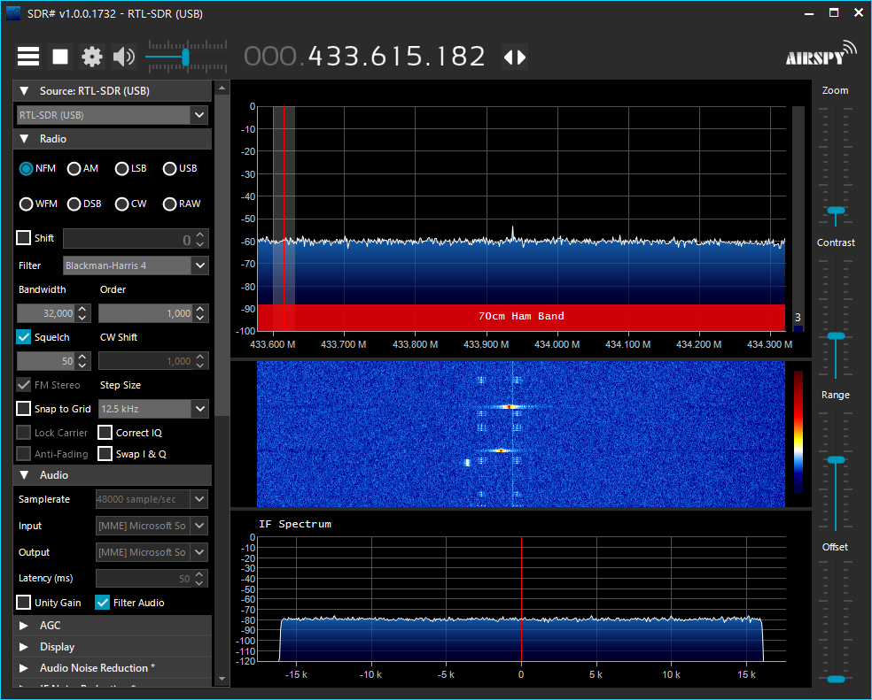
So then I started wondering if it would be possible to decode such signals and it turns out that there is a really awesome command line utility that does exactly this: RTL_433.
RTL_433
So if you have a software defined radio dongle with drivers already installed, and you’re running a debian system (Ubuntu MATE in my case) you can easily install with: apt-get install rtl-433 I believe is it also available for windows but you may have to compile it yourself.
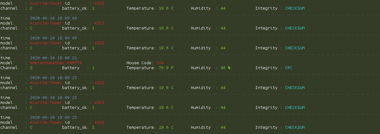
It can be run with rtl-433 in the terminal, with scrolling output.
Or it can be run with some options to output to a file as such:
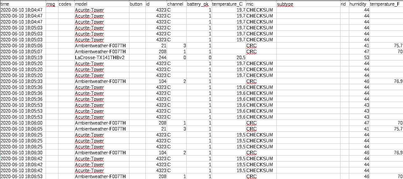
rtl_433 -F csv:weather1.csv
The measurements from my weather station are coming in as Ambientweather-F007TH on channels 1, 2 and 3. As an added bonus, I am also receiving data from some of my neighbors’ weather stations as well!
At first I put a quick script together to read this CSV file with pandas and plot the output. Before plotting, I had to unpivot the data because all the values are output to a single column (either temperature_F or temperature_C). This was fairly painless but then I realized that I wanted to collect data over a long period of time and be able to handle interruptions in data acquisition. Rather than concatenating csv files together, I decided to output the dataframe to an SQLite database. This is easily done with df.to_sql but I found the result to be unsatisfactory due to an issue with appending repeat data to the file. Pandas apparently does not check for existing records and will write the same data over and over again, which could cause the database to grow unnecessarily large.
So then I started on a workaround using SQLite3 to write the data while checking for existing records on a key: 'time'. Below is the quick and dirty workaround that I came up with. It starts off by reading the current csv file into a dataframe and then passes it to a function where the following things take place:
- A connection to the database is created
- A list
DateTimesis created to check for duplicate records in the database- One thing to note, which I found interesting is that RTL_433 outputs a lot of duplicate time stamps. This created a problem when pivoting the data as duplicates in the index are not allowed.
- It counts the columns in the dataframe so that it outputs the right number of values to the table.
- It iterates through the tuples of the dataframe. Sqlite takes the values as nameless tuples.
- it checks if the timestamp (
row[0]) is in theDateTimeslist and if not, inserts the data into the table. - insQmrks is a string like
'?,?,?,?,?'where the number of question marks is the number of columns in the data to be written.
- it checks if the timestamp (
import pandas as pd
import sqlite3
from datetime import datetime
import sys

mydb = 'weather.db'
csvfile = sys.argv[1]

df = pd.read_csv(csvfile, low_memory= False, header=0, index_col=0)

def pd_sqlt(df, mydb, idxcol):
    conn = sqlite3.connect(mydb)
    c = conn.cursor()
    DateTimes = []

    try: #create table if it doesn't exist
        df.to_sql(name='data', con=conn, if_exists='fail')
    except:
        pass

    #Count the columns in the dataframe
    for row in c.execute('SELECT ' + idxcol + ' FROM data'):
        DateTimes.append(row[0])

    #make a string with the correct number of question marks
    insQmrks = '?,' * (len(df.columns) + 1)
    insQmrks = insQmrks[0:len(insQmrks)-1]

    for row in df.itertuples(name=None):
        if row[0] not in DateTimes:
            print('executing' + str(row[0]))
            c.execute('INSERT INTO data VALUES(' + insQmrks + ')', row)

    conn.commit()
    conn.close()

pd_sqlt(df, mydb, 'time')
Read Data & Plot
Now that we’ve collected the data into the sqlite database (perhaps unnecessarily), it’s time to plot and see how it looks. As per my own personal habit, I’ve started a new script for this. We can start by importing some things. Pandas will be needed for data manipulation, matplotlib for plotting, datetime for parsing dates and sqlite3 for reading the SQLite DB.
import pandas as pd
import matplotlib.pyplot as plt
from datetime import datetime
from matplotlib.dates import AutoDateFormatter, AutoDateLocator, DateFormatter
import sqlite3
Let’s take a step back for a minute and explain what we have to do here. The challenge is that the data is coming in like this:
| Time | Channel | Temperature |
|---|---|---|
| 2020-06-10 11:45:00 | 1 | 72.1 |
| 2020-06-10 11:45:10 | 2 | 58.8 |
| 2020-06-10 11:45:34 | 3 | 75.2 |
| 2020-06-10 11:45:46 | C | 73.1 |
| 2020-06-10 11:45:46 | 0 | 74.8 |
What I want to do is plot the temperature from each channel (or device) as a separate series on a chart. So in order to do that, I need the data to look like this:
| Time | 0 | 1 | 2 | 3 | C |
|---|---|---|---|---|---|
| 2020-06-10 11:45:00 | 72.1 | ||||
| 2020-06-10 11:45:10 | 58.8 | ||||
| 2020-06-10 11:45:34 | 75.2 | ||||
| 2020-06-10 11:45:46 | 73.1 | ||||
| 2020-06-10 11:45:46 | 74.8 |
(Assuming each device has a unique channel)
So in order do this we need to use the pandas pivot function. Before I forget however, let’s read the data into a dataframe and parse the dates.
#Connect to the database
conn = sqlite3.connect('weather.db')

#Set up date formatters for the x-axis
xtick_locator = AutoDateLocator()
xtick_formatter = AutoDateFormatter(xtick_locator)

#Set up the date parsing
dateparse = lambda x: datetime.strptime(x, '%Y-%m-%d %H:%M:%S')

#Read the data
df = pd.read_sql('SELECT * from data', con = conn, parse_dates=['time'], \
index_col=['time'])

#Reset the index because of so many duplicate time stamps,
#otherwise pivot will not work.
df.reset_index(inplace=True)
Now we can start doing the pivot,
df0 = df.pivot(columns='channel', values=['temperature_F','time', \
 'temperature_C'])
But that leaves us with a separate time column which is multi-indexed for each channel.
In [7]: df0['time']
Out[7]:
channel NaN   0   1                   2   3                   C channel
0       NaT NaT NaT                 NaT NaT 2020-06-06 22:24:55     NaT
1       NaT NaT NaT                 NaT NaT 2020-06-06 22:24:55     NaT
2       NaT NaT NaT                 NaT NaT 2020-06-06 22:24:55     NaT
3       NaT NaT NaT 2020-06-06 22:25:06 NaT                 NaT     NaT
4       NaT NaT NaT                 NaT NaT 2020-06-06 22:25:11     NaT
...      ..  ..  ..                 ...  ..                 ...     ...
86046   NaT NaT NaT                 NaT NaT 2020-06-11 15:12:59     NaT
86047   NaT NaT NaT                 NaT NaT 2020-06-11 15:12:59     NaT
86048   NaT NaT NaT                 NaT NaT 2020-06-11 15:13:15     NaT
86049   NaT NaT NaT                 NaT NaT 2020-06-11 15:13:15     NaT
86050   NaT NaT NaT                 NaT NaT 2020-06-11 15:13:15     NaT
I ended up doing something kind of messy in order to recombine the time stamps, but it works. It avoids the pandas setting with copy warning error.
df0['time1'] = df0['time']['0']
df0['time2'] = df0['time1'].fillna(df0['time']['1'])
df0['time3'] = df0['time2'].fillna(df0['time']['2'])
df0['time4'] = df0['time3'].fillna(df0['time']['3'])
df0['time5'] = df0['time4'].fillna(df0['time']['C'])

#Get rid of the junk.
df0.drop(labels=['time1', 'time2', 'time3', 'time4'], inplace=True, axis=1)

#Convert C to F for channel 0 and C - the neighbors
df0['X'] = df0['temperature_C']['0'] * (9/5) + 32
df0['Y'] = df0['temperature_C']['C'] * (9/5) + 32
Now we are left with a dataframe with a single column for the time index, with repeating values included. And we also have separate columns for each temperature sensor. Channel 0 and C are from the neighbors.
In [10]: df0[['time5', 'temperature_F']]
Out[10]:
                      time5 temperature_F
channel                               NaN    0    1     2    3     C channel
0       2020-06-06 22:24:55           NaN  NaN  NaN   NaN  NaN  None     NaN
1       2020-06-06 22:24:55           NaN  NaN  NaN   NaN  NaN  None     NaN
2       2020-06-06 22:24:55           NaN  NaN  NaN   NaN  NaN  None     NaN
3       2020-06-06 22:25:06           NaN  NaN  NaN  74.2  NaN   NaN     NaN
4       2020-06-06 22:25:11           NaN  NaN  NaN   NaN  NaN  None     NaN
...                     ...           ...  ...  ...   ...  ...   ...     ...
86046   2020-06-11 15:12:59           NaN  NaN  NaN   NaN  NaN   NaN     NaN
86047   2020-06-11 15:12:59           NaN  NaN  NaN   NaN  NaN   NaN     NaN
86048   2020-06-11 15:13:15           NaN  NaN  NaN   NaN  NaN   NaN     NaN
86049   2020-06-11 15:13:15           NaN  NaN  NaN   NaN  NaN   NaN     NaN
86050   2020-06-11 15:13:15           NaN  NaN  NaN   NaN  NaN   NaN     NaN
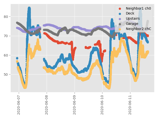
Plot Data
And finally we can do our plotting.
#Start plotting stuff
plt.style.use('ggplot')
fig, ax = plt.subplots()
ax.scatter(df0['time5'], df0['X'], label='Neighbor1 ch0')
ax.scatter(df0['time5'], df0['temperature_F']['1'], label='Deck')
ax.scatter(df0['time5'], df0['temperature_F']['2'], label='Upstairs')
ax.scatter(df0['time5'], df0['temperature_F']['3'], label='Garage')
ax.scatter(df0['time5'], df0['Y'], label='Neighbor2 chC')
ax.xaxis.set_major_locator(xtick_locator)
ax.xaxis.set_major_formatter(xtick_formatter)
plt.xticks(rotation=90)
plt.legend(loc='upper right')
fig.tight_layout()
fig.savefig('weather_v2.png', fig_size=(7, 11))
fig.show()
Next Steps
By gathering this data, I have been able to make some observations that I might not have seen otherwise. The first thing I noticed was that our outside deck sensor gets too hot on sunny mornings, exaggerating the measurement. Then I realized that our garage gets really hot in the afternoons when the sun shines on its door, which (I believe) in turn heats up the upstairs bedrooms excessively at night. I also noticed that when we run an errand and re-park our vehicle inside the garage, the temperature increases immediately. I think I will keep working on this project as I have some ideas to take my learning further:
- Perform some daily descriptive statistics on the data.
- Find the relationship between the temperatures in the different areas of the house.
- Get a raspberry pi for 24/7 data acquisition
- Set up a web server on the pi, using Chart.js to make a dashboard