Well Path Simulator
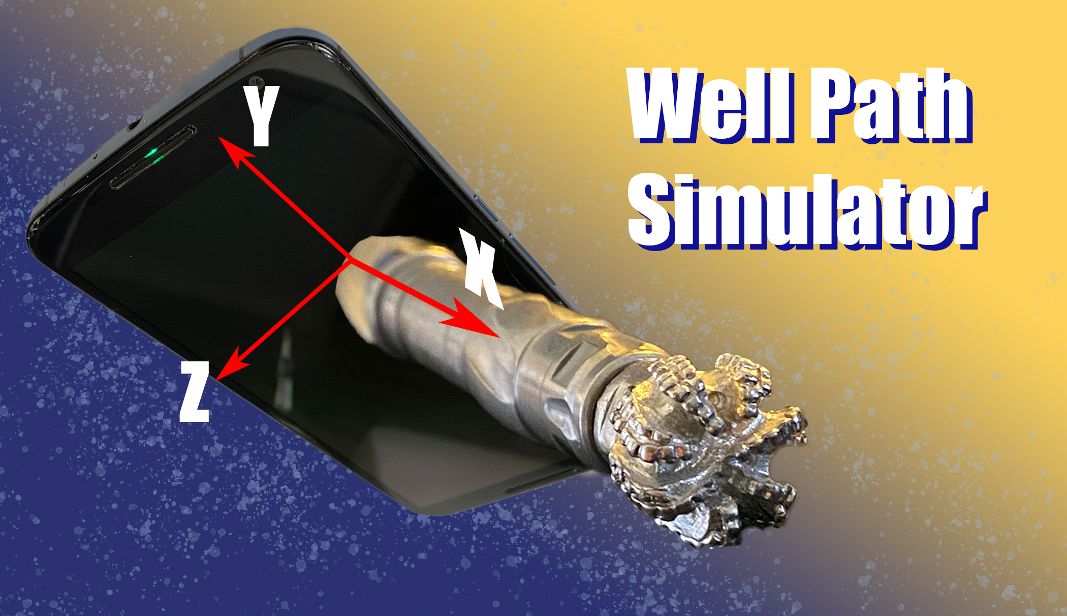
This project is meant to be a fun demonstration of how we can use sensor data from a smart phone in such a way that emulates the real life application of directional drilling in oil & gas wells. Basically, what I want to do is to pretend that I’m drilling a well with my phone in hand, manually controlling the trajectory with the end result being a 3-dimensional plot of the well path along with a set of its surveys. As a drilling engineer, I knew this was possible but had not seen anyone actually do it, so I decided to give it a try.
Sensor Streamer
I found an app called SensorStreamer for my old android phone. It can stream data from the phone’s magnetometers and accelerometers in real time via the local network over UDP in JSON format.
Reading the data from the phone
To read data from the device, I used the python socket module to listen for the data on a port that I specified in the app (8000). In the loop, I used the recv method to read the data. Depending on the buffer size, it sometimes sends in multiple records separated by a new line character \n so I split them out into a list and then filter the list to remove None values. The filter object remains iterable, so I can then load each of the json records from it.
import socket
import json
import time

s = socket.socket(socket.AF_INET, socket.SOCK_STREAM)
#IP Address of phone
host = "192.168.1.4"
port = 8000
buffer_size = 8024
s.connect((host, port))
print("Listening on %s:%s..." % (host, str(port)))

while True:
    data = s.recv(buffer_size)
    mylist = data.decode('utf-8').split('\n')
    mylist = filter(None, mylist) #mylist is now a filter object

    for rec in mylist:
        jdata = json.loads(rec)
        print(jdata)
        time.sleep(1)
Testing this bit of code yields the following output. This is what the JSON records look like. The 3-axis magnetometer and accelerometer readings are included as a nested list in the JSON record.
Listening on 192.168.1.4:8000...
{'accelerometer': {'timestamp': 963062099480427, 'value': [0.08378601, -0.002380371, 9.730026]}, 'magneticField': {'timestamp': 963062117852009, 'value': [-20.129395, -6.564331, -49.739075]}}
{'accelerometer': {'timestamp': 963062290734089, 'value': [0.03590393, -0.07421875, 9.76355]}, 'magneticField': {'timestamp': 963062305352009, 'value': [-21.49353, -5.534363, -50.068665]}}
{'accelerometer': {'timestamp': 963062481987751, 'value': [-0.06463623, 0.007171631, 9.821014]}, 'magneticField': {'timestamp': 963062492852009, 'value': [-20.98236, -7.080078, -49.57428]}}
{'accelerometer': {'timestamp': 963062673271931, 'value': [0.08378601, -0.04069519, 9.662994]}, 'magneticField': {'timestamp': 963062680321492, 'value': [-22.175598, -5.534363, -50.39978]}}
{'accelerometer': {'timestamp': 963062864525593, 'value': [0.08857727, -0.04069519, 9.892838]}, 'magneticField': {'timestamp': 963062867821492, 'value': [-20.300293, -5.3634644, -49.243164]}}
{'accelerometer': {'timestamp': 963063055779255, 'value': [0.06942749, -0.03111267, 9.677353]}, 'magneticField': {'timestamp': 963063055321492, 'value': [-22.175598, -5.8776855, -49.739075]}}
Unpack the JSON to Pandas DataFrame
My first instinct to use the pandas read_json() to read these records resulted in a dataframe with the following structure. I eventually gave up trying to deal with the dataframe in this format.
In [13]: pd.read_json(rec)
Out[13]:
                                         accelerometer                       magneticField
timestamp                             1048967249791200                    1048967333134706
value      [0.04069519, 0.08378601000000001, 9.914383]  [-14.601135, -9.829712, -48.64044]
Rather than try to solve this Rubik’s cube, I essentially just peeled the stickers off and put them in order by directly unpacking the json data into a dictionary and then generated the dataframe from there. See code block below:
def json_rec_to_df(df, mylist):
    for rec in mylist:
        jdata = json.loads(rec)
        df = pd.DataFrame([[jdata['magneticField']['timestamp'],
                            jdata['magneticField']['value'][0]*1000,
                            jdata['magneticField']['value'][1]*1000,
                            jdata['magneticField']['value'][2]*1000,
                            jdata['accelerometer']['timestamp'],
                            jdata['accelerometer']['value'][0]*(1000/9.80665),
                            jdata['accelerometer']['value'][1]*(1000/9.80665),
                            jdata['accelerometer']['value'][2]*(1000/9.80665)]],
                            columns=['btimestamp', 'bx', 'by', 'bz',
                                     'gtimestamp', 'gx', 'gy', 'gz'])
    return df
This results in a much more user friendly dataframe with a separate column for each data point.
Out[25]:
         btimestamp         bx         by         bz        gtimestamp          gx          gy         gz
0  1048879217758634  37123.108 -34417.725 -17448.425  1048879231277921 -664.550433  559.081032  526.85545
Survey Calculation
To calculate the survey (the 3D orientation) involves a bit of magic. These formulas I picked up along-the-way in my previous career, but I should mention that the minimum curvature calculation is easily found with the google search terms “minimum curvature method”. These are the meat and potatoes of this script. The result is a directional survey in the format MD INC AZI TVD NS EW DLS, which is yielded from the raw 6-axis sensor values bx by bz gx gy gz from the device.
- MD: The measured depth, or distance in feet between survey stations
- INC: The inclination of the survey in degrees.
- AZI: The azimuth of the survey in degrees.
- TVD: The true vertical depth of the survey in feet.
- NS: The north/south displacement of the survey.
- EW: The east/west displacement of the survey.
- DLS: A combination of the change of inclination and azimuth, expressed in degrees per 100 ft.
- bx, by, bz: The 3-axis magnetic field components, calculated in nano-Tesla.
- gx, gy, gz: The 3-axis accelerometer (gravity) components, calculated in milli-G.
- G: the magnitude of the gravitational vector, calculated in milli-G.
- B: the total field of the magnetic field vector, also in nano-Tesla.
In the script, I am using the keyboard module to scan for a key press on the space bar such that every time it is pressed, a new survey appears and is added to the list for minimum curvature calculation. Also, since I do not have any drill pipe in my house, I am going to pretend that the survey intervals (MD) are exactly 100 ft.
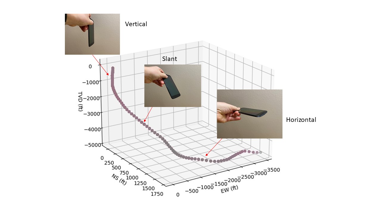
Example Well Path
Here is an example well path that I “drilled” by holding the phone in the desired orientation. Each dot on the plot represents a “survey” that was recorded when I pressed the space bar. First I started out by holding the phone vertical to keep the “surface hole” nice and straight. Then for the “intermediate” section, I increased the angle of the phone and held it there for a while. Finally, in the “production” section, I increased the angle to horizontal (around 90 degrees) while also making a slight turn here and there.
Final surveys:
In [30]: df_final[['MD', 'INC', 'AZI', 'TVD', 'DLS', 'NS', 'EW']]
Out[30]:
      MD        INC         AZI          TVD        DLS           NS           EW
0    100   2.976223  117.410004          NaN        NaN          NaN          NaN
0    200   2.680754  206.193120   -99.917662   3.962197    -3.294833     1.272906
0    300   5.296719  211.297818  -199.667057   2.637375    -9.338303    -2.157713
0    400   2.328175  209.103517  -299.434648   2.971585   -15.058292    -5.544188
0    500   4.227726  201.187211  -399.266940   1.948257   -20.270382    -7.864539
..   ...        ...         ...          ...        ...          ...          ...
0   7400  89.459584  290.415884 -4773.512982  32.801792  1509.208205 -3076.418735
0   7500  90.369228  316.477383 -4773.665001  26.077065  1563.849897 -3159.140135
0   7600  90.584153  299.284380 -4772.826730  17.193737  1625.019971 -3237.770286
0   7700  90.616705  286.812028 -4771.774646  12.471707  1664.091127 -3329.601194
0   7800  90.413187  288.174885 -4770.875865   1.377913  1694.148895 -3424.970167

[78 rows x 7 columns]
Complete Script
See below for the complete script. Let me know if you try it out! In the future, I might input a real well plan and turn it into a directional drilling video game.
import socket
import json
import time
import pandas as pd
import keyboard
import numpy as np
from mpl_toolkits.mplot3d import Axes3D
import matplotlib.pyplot as plt

s = socket.socket(socket.AF_INET, socket.SOCK_STREAM)
host = "192.168.1.4"
port = 8000
buffer_size = 8024
s.connect((host, port))
print("Listening on %s:%s..." % (host, str(port)))

df = pd.DataFrame(columns = ['btimestamp', 'bx', 'by', 'bz'])

dfsrv = pd.DataFrame()
fig = plt.figure()
ax = fig.add_subplot(111, projection='3d')
ax.set_xlabel('EW (ft)')
ax.set_ylabel('NS (ft)')
ax.set_zlabel('TVD (ft)')

def json_rec_to_df(df, mylist):
    for rec in mylist:
        jdata = json.loads(rec)
        df = pd.DataFrame([[jdata['magneticField']['timestamp'],
                            jdata['magneticField']['value'][0]*1000,
                            jdata['magneticField']['value'][1]*1000,
                            jdata['magneticField']['value'][2]*1000,
                            jdata['accelerometer']['timestamp'],
                            jdata['accelerometer']['value'][0]*(1000/9.80665),
                            jdata['accelerometer']['value'][1]*(1000/9.80665),
                            jdata['accelerometer']['value'][2]*(1000/9.80665)]],
                            columns=['btimestamp', 'bx', 'by', 'bz',
                                     'gtimestamp', 'gx', 'gy', 'gz'])
    return df

def survey_calc(df):
    df['G'] = (df['gx']**2 + df['gy']**2 + df['gz']**2)**0.5
    df['B'] = (df['bx']**2 + df['by']**2 + df['bz']**2)**0.5
    df['Dip'] = 90 - np.degrees(np.arccos((df.gx*df.bx + df.gy*df.by + df.gz*df.bz) / \
                                          (df.G*df.B)))
    df['INC'] = np.degrees(np.arccos(df.gx / df.G))
    df['INC'] = abs(df['INC'] - 180) #Flip the axis so it lines up with the azimuth
    df['AZI'] = np.degrees(np.arctan2(df.G*(df.gy*df.bz - df.gz*df.by),
                                      df.bx*df.G**2 - (df.gx*df.bx + df.gy*df.by + \
                                                       df.gz*df.bz)*df.gx)) \
              + np.where((df.gy*df.bz - df.gz*df.by) < 0, 360, 0)
    df['AZI'] = abs(df['AZI'] - 360) #Reverse the values
    return df

def min_curve_calc(MD, I1, I2, A1, A2):
    I1 = np.radians(I1)
    I2 = np.radians(I2)
    A1 = np.radians(A1)
    A2 = np.radians(A2)
    DLS = np.arccos(np.cos(I2 - I1) - (np.sin(I1)*np.sin(I2)*(1-np.cos(A2-A1))))
    RF = (2/DLS) * np.tan(DLS/2)
    NS = (MD / 2) * (np.sin(I1) * np.cos(A1) + np.sin(I2) * np.cos(A2)) * RF
    EW = (MD / 2) * (np.sin(I1) * np.sin(A1) + np.sin(I2) * np.sin(A2)) * RF
    TVD = (MD / 2) * (np.cos(I1) + np.cos(I2)) * RF
    return NS, EW, TVD, DLS, RF

while True:
    data = s.recv(buffer_size)
    mylist = data.decode('utf-8').split('\n')
    mylist = filter(None, mylist) #mylist is now a filter object

    df = json_rec_to_df(df, mylist)
    df = survey_calc(df)

    try:
        if keyboard.is_pressed('space'):
            time.sleep(0.5)
            dfsrv = dfsrv.append(df[-1:])
            dfsrv['MD'] = 100
            print(dfsrv[['MD', 'INC', 'AZI', 'gx', 'gy', 'gz', 'bx', 'by', 'bz']][-1:])
            dfsrv['I1'] = dfsrv['INC'].shift(1)
            dfsrv['A1'] = dfsrv['AZI'].shift(1)
            resdf = dfsrv.apply(lambda x: min_curve_calc(x['MD'],
                                                         x['I1'],
                                                         x['INC'],
                                                         x['A1'],
                                                         x['AZI']),
                                                         axis=1,
                                                         result_type='expand')
            resdf.columns = ['NS', 'EW', 'TVD', 'DLS', 'RF']
            resdf['TVD'] = -resdf['TVD']
            df_final = pd.concat([dfsrv, resdf], axis=1)
            df_final['NS'] = df_final['NS'].cumsum()
            df_final['EW'] = df_final['EW'].cumsum()
            df_final['TVD'] = df_final['TVD'].cumsum()
            df_final['DLS'] = np.degrees(df_final['DLS'])
            df_final['MD'] = df_final['MD'].cumsum()
            ax.scatter(df_final['EW'], df_final['NS'], df_final['TVD'])
            plt.pause(0.5)
    except:
        pass

plt.show()